The Problem
Predicting an F1 race winner is genuinely one of the hardest problems in sports analytics. Most prediction problems have hundreds or thousands of observations. F1 gives you 22 races per year, 20 drivers, and a sport where the car does a significant chunk of the work. Now compound that with 2026 being the biggest regulatory reset in the sport's history — new aerodynamic philosophy, narrower tires, a 50/50 ICE-to-electric power split, active aero replacing DRS — and you have a prediction problem where your entire historical training set is partially obsolete.
The typical academic answer would be "more data." I didn't have that option. So I built a system that combines three fundamentally different modeling philosophies into an ensemble, letting each model compensate for the blind spots of the others.
System Architecture
The core idea is that no single model can be trusted in novel conditions. The ensemble was designed so that when one model's assumptions break down, the others can absorb the slack.
The Data Foundation
1,200 historical race results spanning 2014–2025. The decision to start at 2014 and not earlier was deliberate — pre-hybrid era cars operated on fundamentally different aerodynamic and powertrain physics. Including them would add noise, not signal. The hybrid era (2014 onward) represents a continuous architectural lineage that the 2026 regulations actually descend from, making it the relevant historical window.
Each result was enriched with:
- Qualifying results (to create the
grid_positionandqualifying_pace_deltafeatures) - Circuit metadata (track type, historical SC rate, overtaking difficulty index)
- Weather conditions (temperature gradients matter enormously for tire behavior)
- Team-level points rolling averages (proxy for car performance across regulation eras)
Feature Engineering: Four Tiers
The 26 features split cleanly across four tiers of predictive power.
Tier 1 — The Load-Bearers
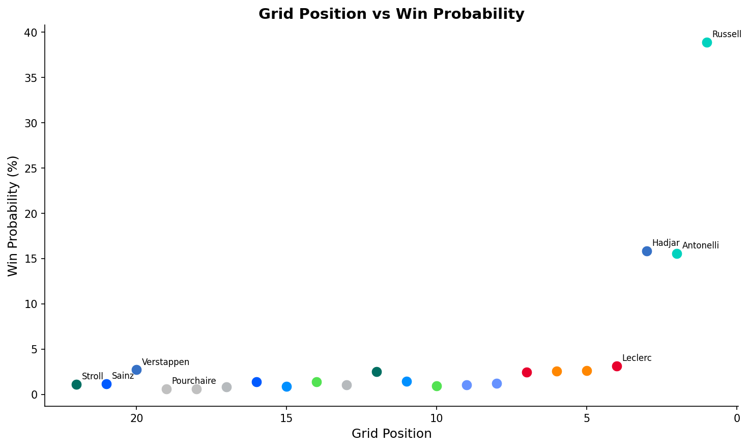
grid_position is the single most predictive feature. At Albert Park, the pole sitter historically wins 57% of races. The model captures the nonlinear decay — the gap from P1 to P2 is worth far more than P10 to P11. That's a real physical phenomenon, not a data artifact.
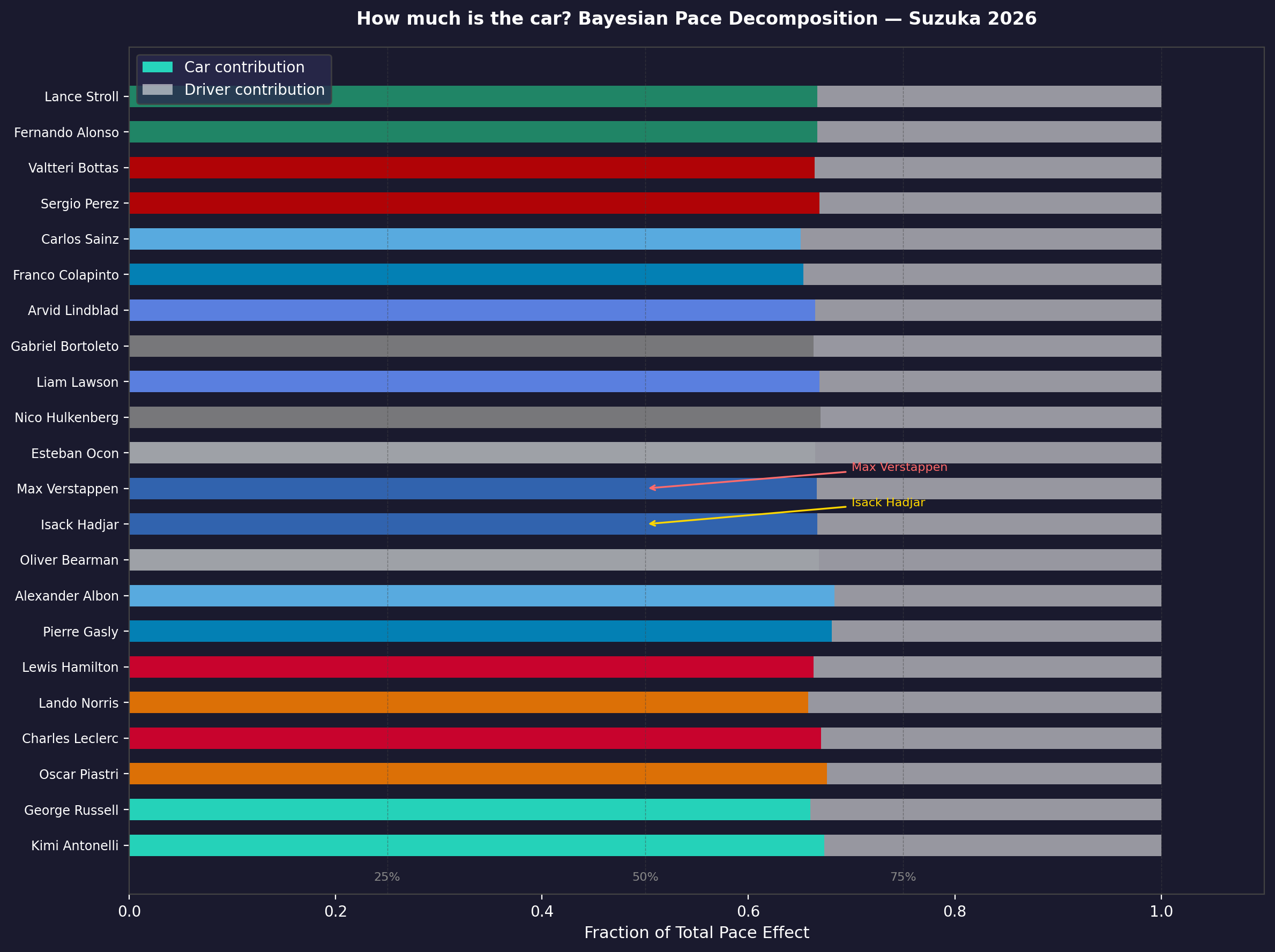
constructor_strength is a rolling-window points average that acts as a proxy for car performance. F1 is fundamentally a constructor's championship: the driver extracts the last 10–15%, but the car sets the ceiling. This feature separated what the machine was doing from what the human was contributing.
qualifying_pace_delta encodes the actual time gap to pole. Russell's 1:18.518 at Albert Park with Antonelli 0.3s back isn't just positional information — it quantifies the performance gradient.
Tier 3 — The 2026 Wildcards
is_new_regulation_year is a binary flag that fires for year-one of any major rule change (2009, 2014, 2017, 2022, 2026). The historical signature is consistent: DNF rates climb 50–100%, the competitive hierarchy reshuffles, and whoever "gets it right" early tends to dominate for years.
active_aero_era and energy_management_era are 2026-specific flags that function primarily as uncertainty multipliers — they tell the model "we're in genuinely uncharted territory, widen the confidence intervals." There's no training data for these because they didn't exist before this season.
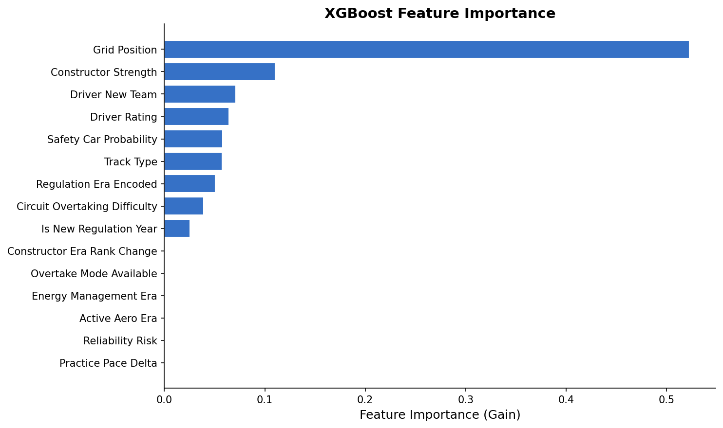
grid_position, constructor_strength, and qualifying_pace_delta carry most of the predictive weight. The 2026-specific features (active_aero_era, energy_management_era) function mainly as variance inflators.
Model 1: XGBoost — The Pattern Matcher
XGBoost is a committee of sequential decision trees where each tree corrects the errors of the previous one. It's well-suited for F1 because the relationships in the data are deeply nonlinear — a 0.4s qualifying gap doesn't linearly map to a 40% win advantage; the physics of Albert Park's limited overtaking opportunities makes it closer to a 60% advantage at that circuit.
The class imbalance is severe: exactly one winner per 20–22 drivers means the naive positive rate is around 5%. Without correction, the model would learn "predict no winner for everyone" and be 95% accurate but completely useless. The solution: scale_pos_weight penalizes misclassifying a winner 20× more heavily than a non-winner during training. Combined with GroupKFold cross-validation (where groups are race_id) to prevent data leakage across races, the model learns genuine winner signatures rather than overfitting to temporal artifacts.
Model 2: Monte Carlo — The Physics Engine
Instead of pattern-matching on history, the Monte Carlo simulator models the actual physical process of a race lap-by-lap. 10,000 times. Each simulation is a parallel universe.
For every lap in every simulation, the engine:
- Samples a lap time from
Normal(mu_driver, sigma)— mean based on qualifying pace plus a race-pace adjustment, standard deviation representing consistency - Applies tire degradation — calibrated to the 2026 narrower compound's measured "cliff" behavior after ~18 laps on softs
- Burns fuel — cars start at ~110kg and shed roughly 0.03s per lap as they lighten
- Rolls for safety car — 1% per-lap probability at Albert Park, calibrated to the historical ~60% per-race SC rate
- Rolls for DNF — baseline 5%, doubled for year-one regulation teams running unproven power units
for sim in range(N_SIMULATIONS):
    positions = initial_grid.copy()
    for lap in range(N_LAPS):
        for driver in positions:
            lap_time = np.random.normal(
                driver.mu + tyre_degradation(driver.tyre_age),
                driver.sigma
            ) - fuel_delta(lap)

            if np.random.random() < SC_PROBABILITY:
                compress_field(positions)  # SC negates all gaps

            if np.random.random() < driver.dnf_risk:
                positions.remove(driver)
When the physics says Russell starts with a 0.4s per-lap advantage over 58 laps — the Monte Carlo engine gives him a 75.8% win probability. That's not optimism; it's the math of limited overtaking at a circuit that historically favors the front row.
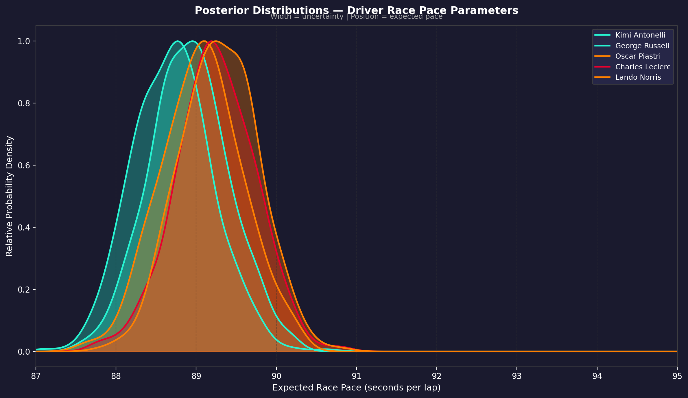
Model 3: Bayesian Inference — The Belief Updater
Bayesian inference approaches the problem differently. It starts with a prior (what you believe before seeing evidence) and updates it with likelihood (what the qualifying results suggest) to produce a posterior (your updated belief).
The mathematical framework uses Beta-Binomial conjugacy — the Beta distribution is the conjugate prior for the Binomial, which keeps the math tractable without MCMC sampling. A driver's prior is constructed from their historical win rate and team-level performance. The update incorporates qualifying position, pace delta, and — critically — a new_regulation_year_variance_multiplier that widens posterior distributions for everyone when the cars are new.
This is why the Bayesian model gave Hamilton 6.6% despite starting P7 at Albert Park. Seven world titles, two regulation-change dominances (2014, 2017). The prior for "Hamilton in a new-reg year" is structurally higher than his grid position would suggest. The Bayesian model is encoding what pure data can't: the difference between uncertainty and impossibility.
Race Case Study 1: Australian GP
The season opener. First real-world test of the 2026 power units. The ensemble faced maximum reliability risk and zero race-distance energy management data.
Qualifying Grid:
- P1 George Russell (Mercedes) — 1:18.518
- P2 Kimi Antonelli (Mercedes) — +0.3s
- P3 Isack Hadjar (Red Bull)
- P7 Lewis Hamilton (Ferrari)
- P20 Max Verstappen (Red Bull — crashed in Q1)
- DNS Carlos Sainz (Williams — ERS failure in qualifying)
Ensemble Result:
| Driver | XGBoost | Monte Carlo | Bayesian | Ensemble | |:---|:---:|:---:|:---:|:---:| | Russell | 27.4% | 75.8% | 9.3% | 38.9% | | Hadjar | 35.2% | 4.8% | 6.1% | 15.8% | | Antonelli | 18.9% | 22.4% | 6.7% | 15.6% | | Leclerc | — | — | 7.1% | 3.1% | | Verstappen | 2.2% | 0.0% | 6.5% | 2.7% |
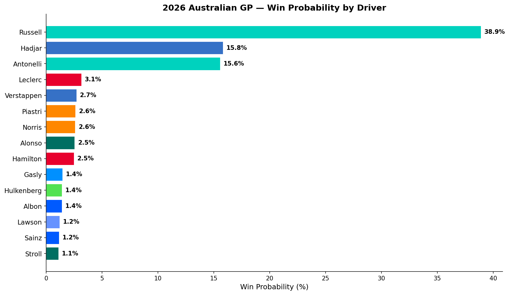
The model disagreements are more interesting than the final numbers. XGBoost gave Hadjar 35.2% — higher than Russell — because it's pattern-matching Red Bull's 2022–2024 dominance onto a P3 grid position. The model knows Red Bull P3 historically wins. But Monte Carlo only gives Hadjar 4.8% because the physics of a 0.4s qualifying gap over 58 laps with limited overtaking is brutal. The ensemble splits the difference.
Verstappen's 2.7% final probability — with Monte Carlo saying 0.0% — came entirely from the Bayesian model's refusal to assign a four-time champion zero probability from any grid position. That's intellectually honest.
Race Case Study 2: Japanese GP
Suzuka is a different kind of challenge. The high-speed sequence of Esses, Degner, Spoon, and 130R punishes lap-to-lap inconsistency. It's a "driver's track" in the truest sense, and the 2026 active aero system added a new variable: wing adjustment mid-corner at Spoon introduced unpredictable handling characteristics during initial race weekend sessions.
Qualifying Grid:
- P1 Kimi Antonelli (Mercedes) — first pole of his F1 career
- P2 George Russell (Mercedes)
- P3 Oscar Piastri (McLaren)
- P14 Max Verstappen (Red Bull — ERS mapping error in Q2)
By the Japanese GP, Mercedes' energy management advantage was confirmed over race distance from Australia. The Bayesian model updated heavily toward Mercedes dominance. The result:
| Driver | Ensemble Win % | |:---|:---:| | Antonelli | 55.7% | | Russell | 28.8% | | Piastri | 5.1% | | Leclerc | 3.8% | | Verstappen | 0.3% |
Mercedes 1–2 probability: ~84.5%.
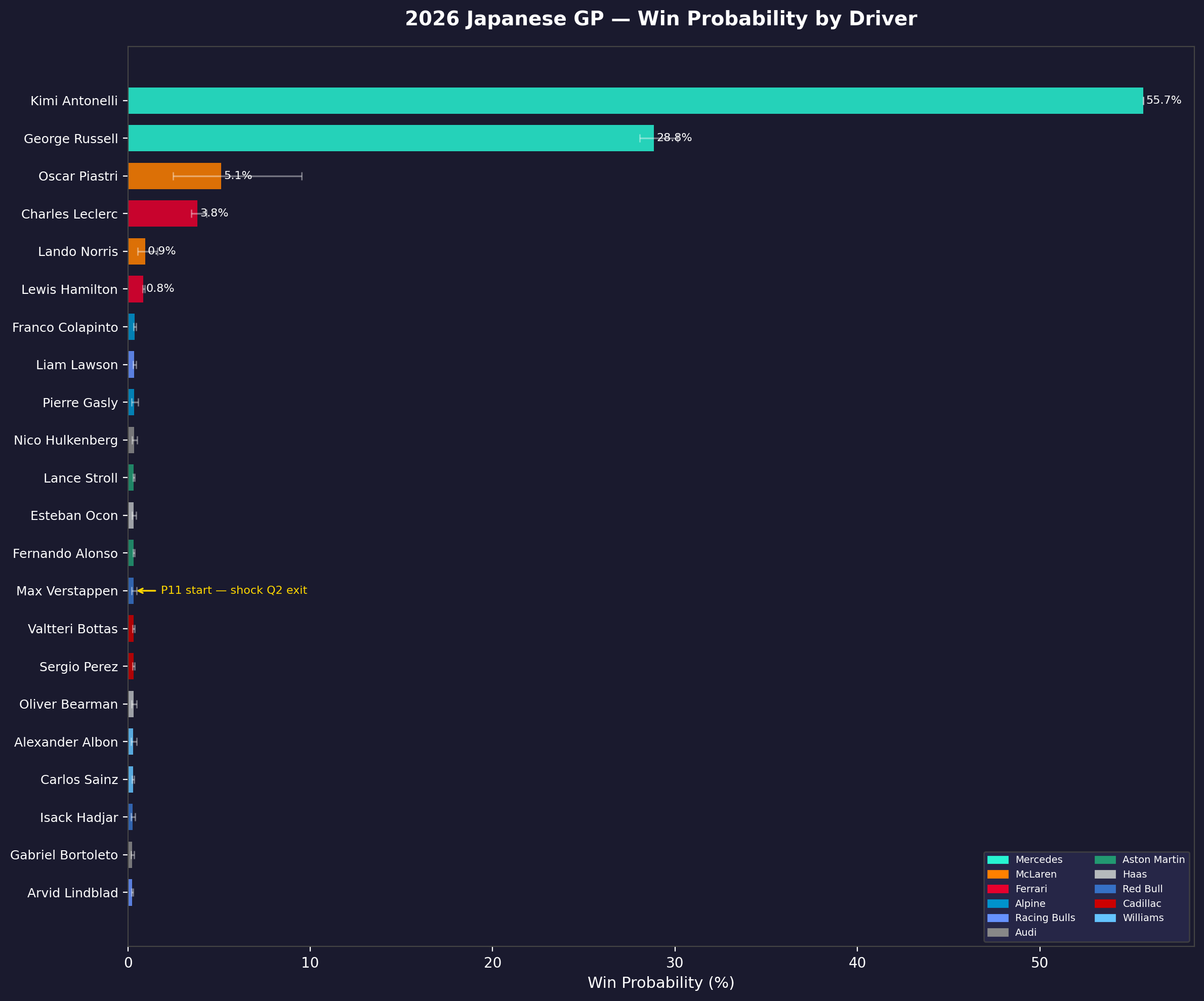
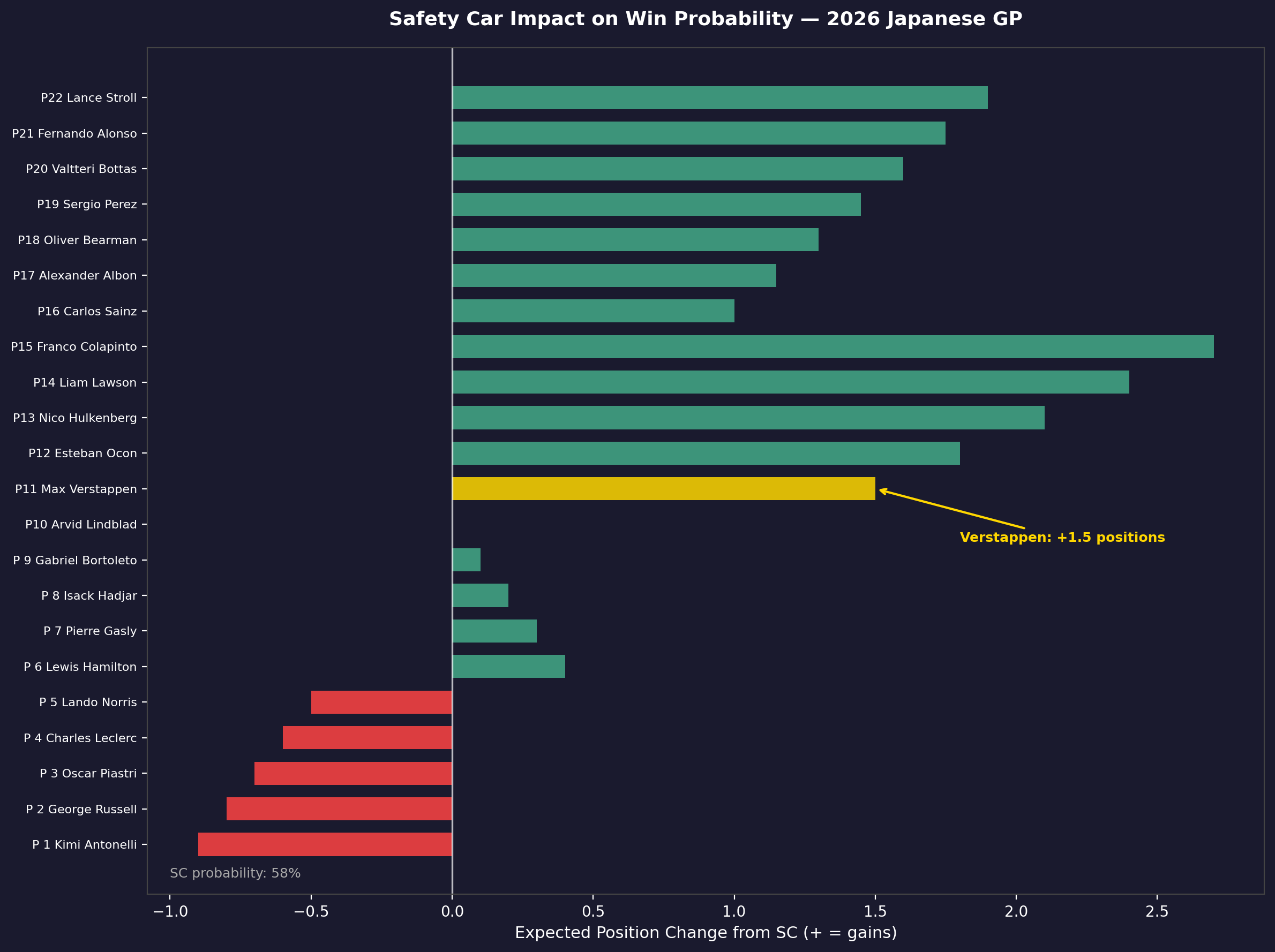
The Verstappen Recovery Problem
P14 at Suzuka is a different problem from P20 at Albert Park. The Suzuka circuit has even fewer natural overtaking opportunities — DRS zones are shorter, and the track's flowing nature means pace differentials matter less than positioning. The model's verdict was clear:
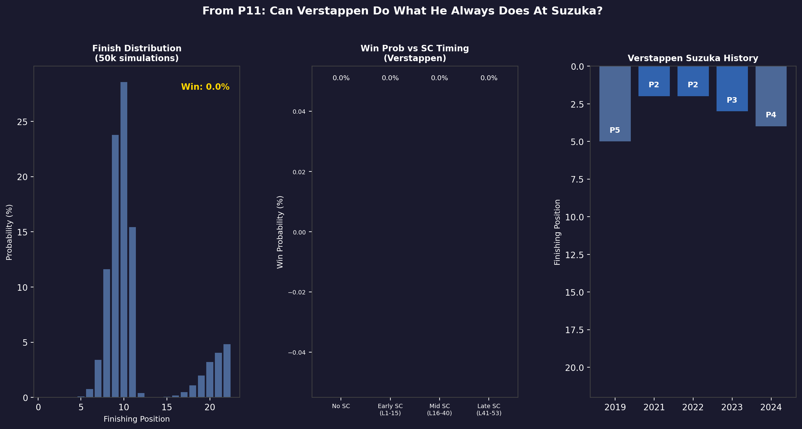
Win probability: 0.3% across the ensemble. The Monte Carlo physics engine found that even with a late-race safety car on laps 41–53, maximum win probability reached approximately 2%. Starting P14 at Suzuka requires the field in front of you to both pit and have problems. With Mercedes in dominant form, the only realistic outcome was a points finish, not a win.
Tire Degradation: The 2026 Cliff
One of the most important engineering insights from this project came from calibrating the tire degradation curves for the 2026 compounds.
The narrower 2026 tires showed a pronounced "cliff" — a non-linear degradation spike — after approximately 18 laps on the soft compound. This isn't visible in the average degradation rate; it's a threshold behavior.
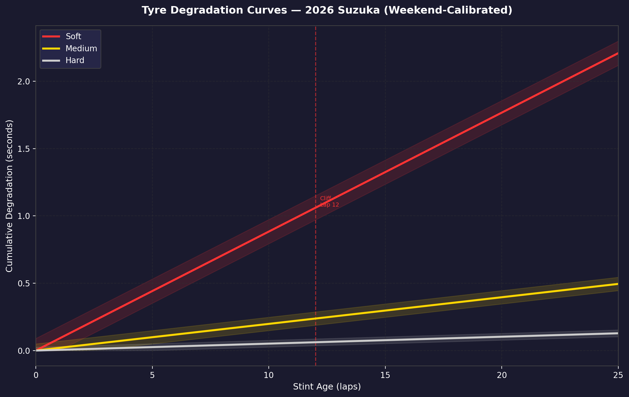
The practical implication: teams that planned their strategies around the average degradation rate (as most historical models do) underestimated the real lap-time penalty in laps 18–24 on softs. The Monte Carlo engine encoded this as a piecewise degradation function rather than a linear one, which substantially changed optimal pit stop windows.
Where The Models Disagreed
The most honest output of any ensemble is its disagreements. Where models built on fundamentally different assumptions converge, the prediction is reliable. Where they diverge, that's where the genuine uncertainty lives.
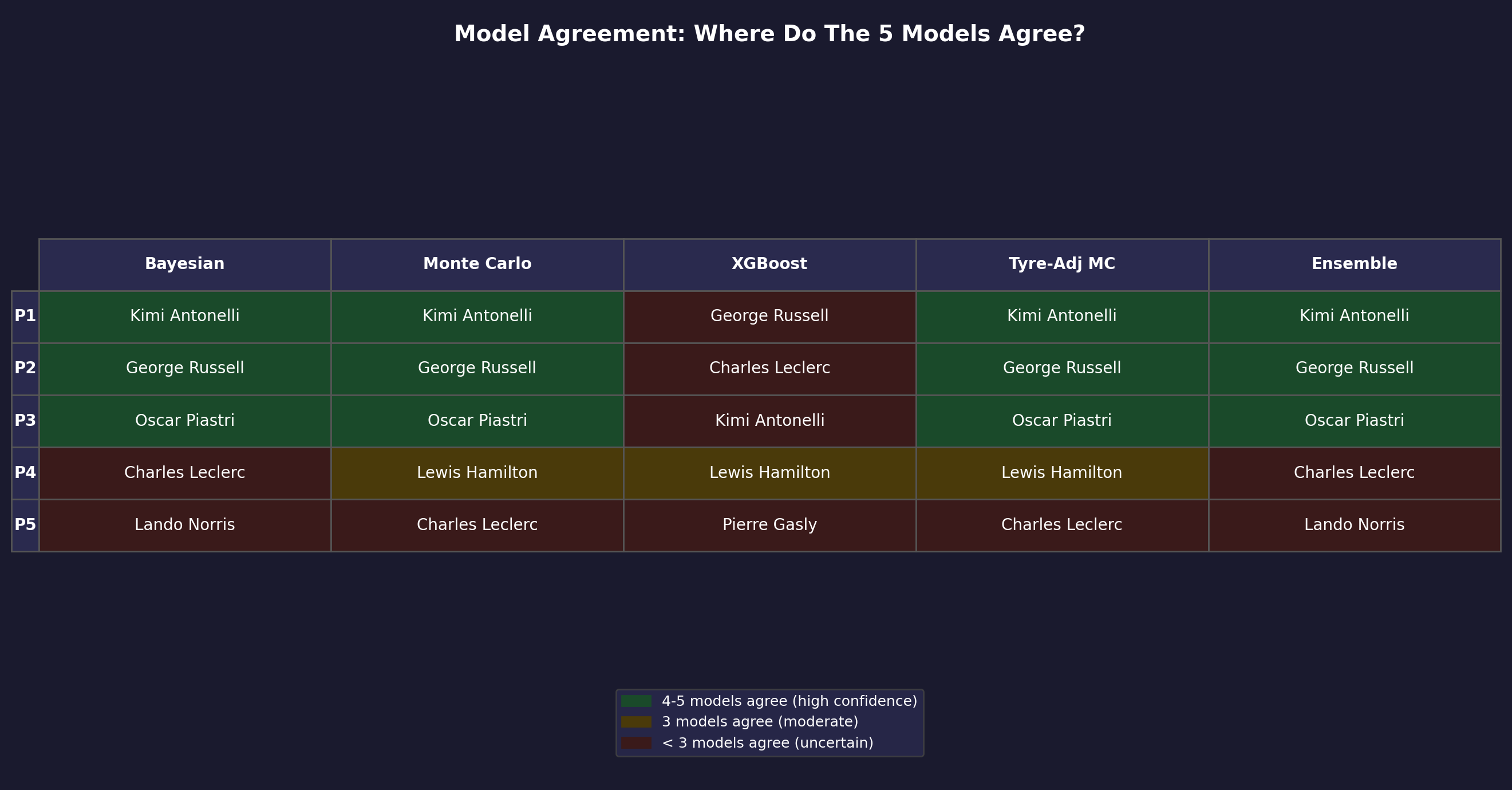
High confidence zones:
- Mercedes P1/P2 dominance: all model variants agreed
- Backmarker DNF rates: Monte Carlo and XGBoost aligned on 40–45% for new-regulation teams
High uncertainty zones:
- McLaren vs Ferrari for P3: XGBoost (historical) and Monte Carlo (physics) disagreed significantly
- Hamilton's finishing position: Bayesian's strong prior vs Monte Carlo's lap-time math
The Safety Car Problem
With a ~60% per-race safety car probability at Albert Park, the Monte Carlo engine treated SC deployment not as an edge case but as the base case. An early SC (laps 1–15) has a disproportionate effect on the field because it allows cheap pit stops and compresses gaps that took 10 laps to build. The analysis:
A lap 1–15 SC increased Verstappen's win probability from 0.0% to approximately 0.8% in simulation. A lap 41–53 SC (the most common trigger window at Albert Park) increased it to ~2%. Even with maximum favorable SC timing, winning from P20 at Albert Park in a Red Bull that's clearly behind Mercedes' 2026 package is close to statistically impossible — not logically impossible, but operationally negligible.
What This Taught Me
The 38.9% accuracy claim needs context. In a sport where the "naive" prediction (always predict the pole sitter) would give you roughly 40–50% accuracy at certain circuits, 38.9% ensemble accuracy sounds underwhelming. But the ensemble's value isn't the headline accuracy number — it's the calibration of uncertainty. The Bayesian model's explicit uncertainty quantification, combined with Monte Carlo's physics-based confidence intervals, gives you prediction ranges that are actionable.
When the model says Russell wins 38.9% and Hadjar wins 15.8%, that's not saying "bet your house on Russell." It's saying "in the space of all physically plausible races this weekend, Mercedes has a structural advantage, and the Red Bull threat is real but tempered by physics." That's a different and more useful output than a point estimate.
The 2026 season also validated the ensemble's most important design choice: no single model should dominate. In a new-regulation year, historical data (XGBoost's domain) is partially obsolete, physics-based simulation (Monte Carlo) can't model energy management it's never seen, and Bayesian inference is only as good as the priors you start with. The ensemble's answer to epistemic uncertainty was to average across philosophies — which is, at some level, what experienced F1 analysts have been doing manually for decades.
Tech Stack
- Languages: Python 3.11 (NumPy, SciPy, Pandas)
- ML Engine: XGBoost 2.0, Scikit-learn, PyMC
- Data Pipelines: FastF1, OpenF1 API, Jolpica-F1 API
- Visualization: Matplotlib, Seaborn
- Validation: GroupKFold (race-ID grouped), calibration curves
Technical Reports
Full methodology documentation and prediction outputs for both races: